scGCO
Recently, I read a fantastic literature about finding SVGs through HMMF and graph cuts algorithm named Identification of spatially variable genes with graph cuts.
Part1
Firstly, we must figure out why finding SVGs is critical in spatial transcriptomics?
Firstly, SVGs are defined as genes whose expression distributions display significant dependence on their spatial locations.
Part1
In this paper, it mentions three reasons:
1、SVGs could demonstrate strong conservation in their spatial patterns, such that many SV genes display similar dependencies on spatial locations, resulting in similar trends in spatial patterns of their expression values.
2、SVGs are often markers or essential regulators for tissue pattern formation and homeostasis.
3、Although these methods demonstrated usefulness in identifying SV genes, they cannot illustrate the exact boundaries of regions demonstrating spatial dependence, which are often of biological interest, and more importantly, these algorithms have computational efficiency of O(n2)orworseandareunsuitable for analyzing large spatial transcriptomics datasets.
Part2
How does this paper identify SVGs?
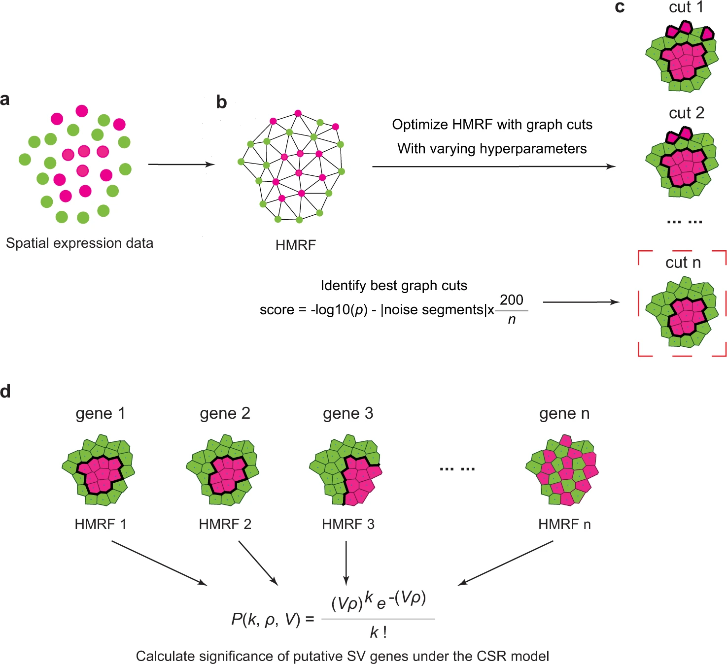
As the above picture illustrated, firstly, to model the spatial gene expression data with HMRF, scGCO first employs Delaunay triangulation to transform spatial locations of measured cells/spots into an undirected graph, where each node represents a data point (a single cell or a spot measuring multiple cells, depending on the technologies utilized) in the spatial transcriptomics data.
Secondly, scGCO utilizes Gaussian mixture modeling to separate a gene’s expression values into different bins, which represent different gene expression states. The float gene expression value associated with each node in the HMRF was then transformed into the corresponding bin number, and the resulting bin number was assigned to the node, creating an initial label assignment for the HMRF.
Thirdly, The initialized HMRF was then optimized by the fast graph cuts algorithm of Boykov to learn the true hidden labels of the nodes in HMRF, which represent authentic gene expression states.
Fourthly, the p-value for each gene was evaluated using the best segmentation under the complete spatial randomness (CSR) framework. Benjamini–Hochberg (BH) correction was utilized to identify spatially variable (SV) genes at the genome-scale.