SOMDE
Recently, I read a paper to identify spatial variable genes named "SOMDE: a scalable method for identifying spatially variable genes with self-organizing map."
Part1
As its abstract shows:
We present SOMDE, an efficient method for identifying SVgenes in large-scale spatial expression data. SOMDE uses the self-organizing map to cluster neighboring cells into nodes and then uses a Gaussian process to fit the node-level spatial gene expression to identify SVgenes. Experiments show that SOMDE is about 5–50 times faster than existing methods with comparable results. The adjustable resolution of SOMDE makes it the only way to give results in 5 min in large datasets of more than 20 000 sequencing sites. SOMDE is available as a python package on PyPI at https://pypi.org/project/somde for educational use.
So, what is the self-organizing map?
A self-organizing map (SOM) is a type of artificial neural network (ANN) that is trained using unsupervised learning to produce a low-dimensional (typically two-dimensional), discretized representation of the input space of the training samples, called a map, and is therefore, a method to make dimensionality reduction. Self-organizing maps differ from other artificial neural networks as they apply competitive learning instead of error-correction education (such as backpropagation with gradient descent) because they use a neighborhood function to preserve the topological properties of the input space.
Part2
And, how does it work in the paper?
Let us see this figure.
\(N^2 \times k=C\)
where C is a constant representing the total number of data sites, and k is the model parameter called the neighbor number, which denotes the expected average number of original data sites each SOM node represents. This parameter controls how condensed the learned SOM is. A larger k means higher condensation.
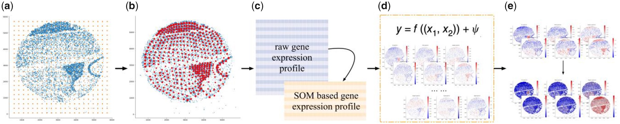
As it showed in (a), it initializes the value and dimension of SOM Node weight \(M=(m_1,m_2,m_{N*N})\) , like the orange spots. After initialization, SOM adjusts the weight of each node toward the tissue spatial topology through a repetitive training process using all spatial coordinates \(X=(X_1,X_2,X_3,X_C)\) as tranining samples.
Cycle after cycle. After training, each data site maps to a unique SOM node. Each SOM node represents the group of sites that are mapped to it. Node weights in the learned SOM can be treated as new spatial coordinates for the data sites. The new spatial locations \(X=\left(\tilde{x}_1, \tilde{x}_2, \ldots, \tilde{x}_{N \times N}\right)\) compose the sparse topology of the original data
In a SOM node, to define its gene expression as the linear combination of the max value and average value of the gene expression in the group of sites that the node represents. The reason for not using average value as a meta-expression is due to the high sparsity in large-scale data that could bias the result.
\(\tilde{\boldsymbol{Y}}_{i, j}=\gamma \cdot \max \left(y_{S 1}, y_{S 2}, \ldots\right)+(1-\gamma) \cdot \operatorname{avg}\left(y_{S 1}, y_{S 2}, \ldots\right)\)
where \(y_{S 1}\) is the expression value of the gene at the data site \(x_{S 1}\). The combination ratio \(\gamma\) balances the local maximum and mean gene expression. We use \(\gamma = 0.5\) as the default in current experiments.
With this computational model, how to deduce SVGs?
\(p\left(\tilde{\boldsymbol{y}} \mid H_{\mathrm{G}}, \tilde{\boldsymbol{X}}, \Theta\right)=\mathcal{N}\left(\tilde{\boldsymbol{y}} \mid \mu \cdot 1, \sigma_s^2 \cdot \boldsymbol{\Sigma}_{k(\tilde{\boldsymbol{x}}, \widetilde{\boldsymbol{x}} \mid \theta)}+\delta \cdot \boldsymbol{I}\right)\)
where \(\tilde{\boldsymbol{y}}\) denotes one gene meta-expression in the SOM plane and \(\tilde{\boldsymbol{X}}\) denotes SOM node locations.
\(\delta \cdot \boldsymbol{I}\) indicates the non-spatial variance given by Gaussian distributed noise in all observed gene meta-expressions. \(\boldsymbol{\Sigma}_{k(\tilde{\boldsymbol{x}}, \widetilde{\boldsymbol{x}} \mid \theta)}\) captures the spatial variation by using a selected kernel function \(k(\cdot)\)
Compared with the original Gaussian process model, model HG assumes one gene meta-expression at all spatial locations has the same mean value l so that the non-spatial variance cannot be regressed out. Thus the maximum likelihood value of HG mainly depends on spatial variance.