SpatialDE
To some degree, SpatialDE is the first literature focused on spatial variable genes(SVGS).
Now, I would like to intriduce the algorithm principle.
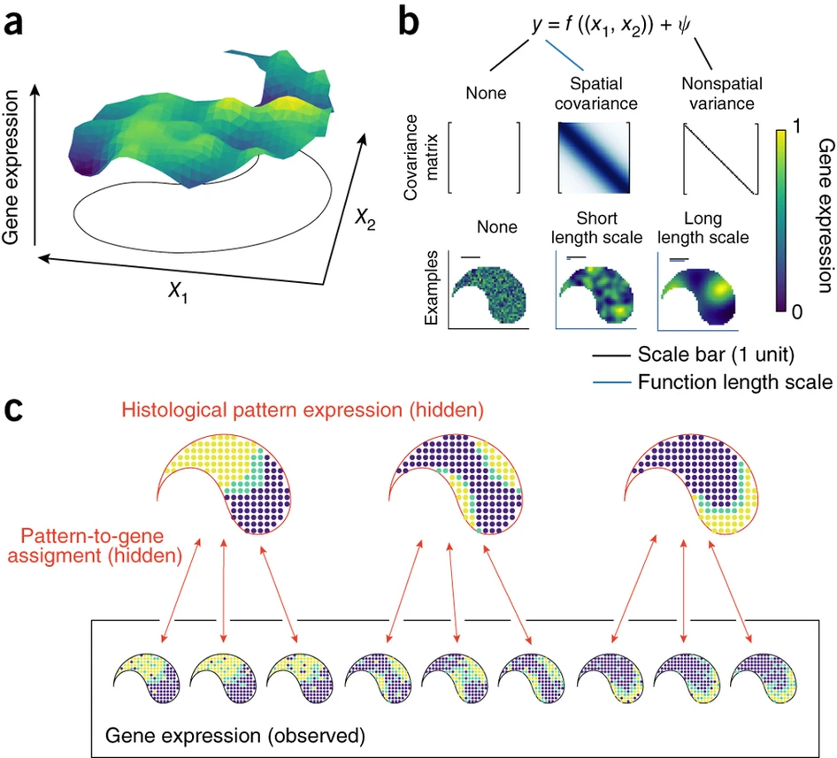
Its method depend on Gaussian process regression. For each gene, SpatialDE decomposes expression variability into spatial and nonspatial components, using two random effect terms: a spatial variance term that parametrizes gene expression covariance by pairwise distances of samples, and a noise term that models nonspatial variability.
\(P\left(y \mid \mu, \sigma_s^2, \delta, \Sigma\right)=N\left(y \mid \mu \cdot 1, \sigma_s^2 \cdot(\Sigma+\delta \cdot I)\right)\)
\(y\) represents the observed gene expression levels, \(μ\) represents the mean expression level, \(\sigma_s^2\) represents the variance of the expression levels, \(δ\) represents the spatial variance, and \(Σ\) represents the covariance matrix of the spatial coordinates.
\(\Sigma_{i, j}=k\left(x_i, x_j\right)=\exp \left(-\frac{\left|x_i-x_j\right|^2}{2 \cdot l^2}\right)\)
\(x_i\) and \(x_j\) represent the spatial coordinates of two locations, and \(l\) is a parameter that determines the scale of the distance over which the similarity between the locations is calculated. The function calculates the similarity between the two locations as a value between 0 and 1, with higher values indicating greater similarity.
The second covariance term \(δ ·I\) accounts for independent nonspatial variation in gene expression, where the ratio \(1/(1 + δ)\) can be interpreted as the fraction of expression variance attributable to spatial effects. Model parameters are fit by maximizing the marginal log likelihood (LL)
\(\begin{aligned} L L= & -\frac{1}{2} \cdot N \cdot \log (2 \pi)-\frac{1}{2} \cdot \log \left(\left|\sigma_s^2 \cdot(\Sigma+\delta \cdot I)\right|\right) \\ & -\frac{1}{2} \cdot(y-\mu \cdot 1)^T\left(\sigma_s^2 \cdot(\Sigma+\delta \cdot I)\right)^{-1}(y-\mu \cdot 1)\end{aligned}\)
To estimate statistical significance, it compared the model likelihood of the fitted SpatialDE model with the likelihood of a model that corresponds to the null hypothesis of no spatial covariance,
\(P\left(y \mid \mu, \sigma^2\right)=N\left(\mu \cdot 1, \sigma^2 \cdot I\right)\)
Then estimating P values analytically on the basis of the χ2 distribution transformation with one degree of freedom.