SPARK
What is SPARK?
SPARK directly models spatial count data through generalized linear spatial models. It relies on recently developed statistical formulas for hypothesis testing, effectively controlling type I errors and yielding high statistical power.
This literature thinks there are three disadvantages in the two existing approaches to identifying spatial variable genes(SVGs).
Firstly, SpatialDE and Trendsceek transform count data into normalized data, which may fail to account for the mean-variance relationship in raw counts.
Secondly, SpatialDE relies on asymptotic normality and minimal P-value-combination rules for constructing hypothesis tests which may cause many true SVGs ignored.
Thirdly, like Trendsceek, its module is not efficient which causes amounts of calculation time.
SPARK's principle
Now, I would like to choose the SPARK principle.

It builds upon a generalized linear spatial model (GLSM) with a variety of spatial kernels to accommodate count data generated from smFISH or sequencing-based spatial transcriptomics studies. With a newly developed penalized quasi-likelihood (PQL) algorithm, SPARK is scalable to analyzing tens of thousands of genes across tens of thousands spatial locations. Importantly, SPARK relies on a mixture of χ2 distributions to serve as the exact test statistics distribution and takes advantage of a recently developed Cauchy combination rule to combine information across multiple spatial kernels for calibrated P value calculation. As a result, SPARK properly controls for type I error at the transcriptome-wide level and is more powerful for identifying SE genes than existing approaches.
\(y_i\left(s_i\right) \sim \operatorname{Poi}\left(N_i\left(s_i\right) \lambda_i\left(s_i\right)\right), i=1,2, \cdots, n\)
\(y_i\left(s_i\right)\) as the gene expression measurement in terms of counts for the i’th sample.
\(N_i(s_i)\) as the normalization factor for i'th sample. Here, it set \(N_i(s_i)\) as the summation of the total number of counts across all genes for the sample as the main interest is in analyzing the relative gene expression level.
\(\log \left(\lambda_i\left(s_i\right)\right)=\boldsymbol{x}_i\left(s_i\right)^{\boldsymbol{T}} \boldsymbol{\beta}+b_i\left(s_i\right)+\epsilon_i\)
where \(\lambda_i\left(s_i\right)\) is an unknown Poisson rate parameter that represents the underlying gene expression level for the i'th sample. In the spatial setting, \(\lambda_i\left(s_i\right)\) can also be viewed as the unobserved spatial random process occurring at location \(𝒔_𝑖\). We model the log scale of the latent variable \(\lambda_i\left(s_i\right)\) as a linear combination of three terms.
\(\log \left(\lambda_i\left(s_i\right)\right)=\boldsymbol{x}_i\left(s_i\right)^T \boldsymbol{\beta}+b_i\left(s_i\right)+\epsilon_i\)
\(x_i\left(s_i\right)\) is k-vector of covariates that include a scalar of one for the intercept and k-1 observed explanatory variables for the i'th sample.
𝜷 is a k-vector of coefficients that include an intercept representing the mean log-expression of the gene across spatial locations together with k-1 coefficients for the corresponding covariates; ∈𝑖 is the residual error that is independently and identically distributed from 𝑁(0,\(𝜏^2\)) with variance \(𝜏^2\); and \(𝑏_𝑖(𝒔_𝑖)\) is a zero-mean, stationary Gaussian process modeling the spatial correlation pattern among spatial locations
\(\boldsymbol{b}(s)=\left(b_1\left(s_1\right), b_2\left(s_2\right), \cdots, b_n\left(s_n\right)\right)^T \sim \operatorname{MVN}\left(0, \tau_1 \boldsymbol{K}(s)\right)\)
The covariance \(K(s)\) is a kernel function of the spatial locations 𝒔=(𝒔1,…,𝒔𝑛)𝑇, with ij’th element being 𝑲(\(𝒔_𝑖\),\(𝒔_𝑗\)); 𝜏1 is a scaling factor of the covariance kernel; and MVN denotes a multivariate normal distribution.
This is the defined GLSM model.
testing whether a gene shows spatial expression pattern can be translated into testing the null hypothesis \(𝑯_0\):𝜏1=0. The statistical power of such a hypothesis test will inevitably depend on how the spatial kernel function \(K(s)\) matches the true underlying spatial pattern displayed by the gene of interest.
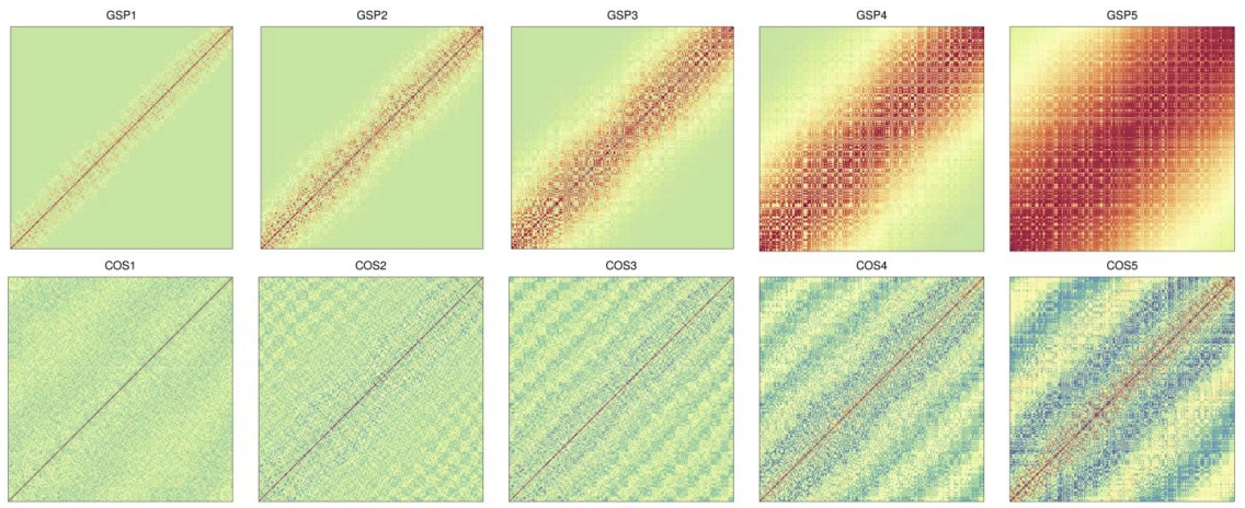
The true underlying spatial pattern for any gene is unfortunately unknown and may vary across genes. To ensure robust identification of SE genes across various spatial patterns, SPARK considers using a total of ten different spatial kernels, including five periodic kernels with different periodicity parameters and five Gaussian kernels with different smoothness parameters.

How to calculate the p-value
First, SPARK tests the null hypothesis using the ten kernels one at a time. By one designed algorithm, to get the p-value. Afterward, it combines these ten p-values through the recently developed Cauchy p-value combination rule. To apply the Cauchy combination rule, we convert each of the ten p-values into a Cauchy statistic, aggregate the ten Cauchy statistics through summation, and convert the summation back to a single p-value based on the standard Cauchy distribution, because the Cauchy rule takes advantage of the fact that combination of Cauchy random variables also follows a Cauchy distribution regardless whether these random variables are correlated or not